ripr computes reverse information projections onto nulls that take the form of a union of convex parts, and then proves an upper bound on the expectation over the null of whatever random variable you get. The projection is fitted via variants of Frank–Wolfe (Jaggi 2013) and/or expectation-maximisation; bounds are proved by a branch-and-bound algorithm (currently for multinomial families, via the Bernstein enclosure of Garloff (1985) and Leroy (2012)). At the end, you get a random variable that is genuinely an e-variable for the null.
Fitting and certification are deliberately separate: any approximate projection can be rescaled (by an upper bound on the expectation over the null) to get a valid e-variable. This way, a very difficult, non-convex optimisation problem splits into two easier problems: approximate a distribution, then compute a bound. The better the fit, the higher the e-power, and validity is guaranteed.
The usual workflow
Take a three-category multinomial distribution (n = 20 samples) and the plurality null: candidate 1 does not win outright, H0 = union_j {theta : theta_1 <= theta_j}. This null is a union of two convex parts, so it’s built with |:
library(ripr)

K <- 3L
n <- 20L
family <- multinomial_family(n_trials = n, k = K)

# Defines {theta : theta_1 <= theta_j}
plurality_part <- function(j) {
  vertices <- diag(K)
  vertices[1L, ] <- replace(numeric(K), c(1L, j), 0.5)
  simplex_region(vertices = vertices)
}

plurality <- null_model(
  family,
  plurality_part(2) | plurality_part(3)
)
We nominate a discrete mixture-multinomial alternative (here a single dirac at q = (0.40, 0.35, 0.25)), so Q is just Multinomial(20, q):
Fitting is a sequence of step verbs: e.g. sfw_step() for sliding Frank–Wolfe, em_step() for EM. Here we run sliding Frank–Wolfe for (at most) 10 iterations, then ripr_finish() extracts the fit:
set.seed(1)
state <- ripr_init(Q, plurality)
state <- sfw_step(state, times = 10L, until = gap_below(1e-10))
fit <- ripr_finish(state, correct_weights = TRUE, record_gap = TRUE)

c(kl = fit@kl, gap = fit@gap_final, atoms = n_atoms(fit@W0))
#>         kl        gap      atoms
#> 0.02822068 0.00000000 2.00000000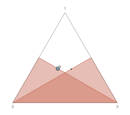
Plurality null, with the support of the alternative mixing distribution W1 and the fitted null mixture W0.
The fit gives a candidate e-variable: the mixture likelihood ratio Q / P*. random_variables are callable, mapping outcomes to their realisation:
X <- likelihood(Q, label = "Q") /
  likelihood(fit@P_star, label = "P*")

outcomes <- rbind(
  c(10L, 10L, 0L),
  c(8L, 7L, 5L)
)
X(outcomes)
#> [1] 0.8372139 1.0794622
certify() proves an upper bound on expectation of X over the null, including a lower-bound that is the largest value the search actually attained:
cert <- certify(X, plurality, tol = 1e-9)
cert
#> <ripr_certificate>
#>   X = Q / P*
#>   under null_model: multinomial_family over 2 parts
#>   sup E[X] <= 1  (certified via bernstein)
#>   sup E[X] >= 1  (interval width: 9.46e-10)
#>          bound attained iterations converged
#>   part 1     1        1         26      TRUE
#>   part 2     1        1         28      TRUE
#>   e_variable(): X / 1
Rescaling by the upper bound turns X into a bona fide e-variable for the plurality null, which is what e_variable() does with a certificate:
E <- e_variable(cert)
print(E)
#> <random_variable> Q / P* / 1
#>   on count_space, dimension 3
print(E(outcomes))
#> [1] 0.8372139 1.0794622
Learn more
vignette("ripr") walks through the same example in more depth: why validity survives a deliberately bad fit, how a bound from certify() differs from sup_lb(), and what happens when no certification method exists for a family/geometry pair. vignette("regions") covers the region interface and set algebra (|, &, -, == and disjoin()) used to build nulls out of convex pieces.